Simple Spatial Experiments

The project described here is a simple data recording program for the Phidget Spatial. We play with the program and record data to learn things about our environment.

Practical concepts covered are (click on links to see other projects on that topic): Data Logging Writing to a text file Using Phidgets with C/C++ Analyzing your Phidget Data

As with any of our described projects, Phidgets takes care of the electrical component design. Here, we also provide some simple code so you can play around with your Spatial and save the data to plot later.

Time: About two hours

Special Needed Tools: A Phidget Spatial, USB cord, and your computer.

• You should have already worked through our Phidget Spatial Getting Started Guide for your Spatial Device - this will show you how to get the the Phidget Libraries installed for your operating system.
• Your computer should have a C compiler we support (including gcc, MinGW, Borland, Visual Studio, and many more)
• If you would like to follow along with the graphing examples, you can install the R Statistical package, which is free and available for Windows, Mac, and Linux.

Introduction

A Phidget Spatial can measure acceleration, and some models can also measure gyroscopic motion and magnetic fields.

We start with a Phidget spatial just on our desk, and then play around with it and plot the data.

Phidgets

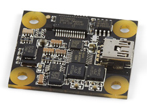
All you need is a Phidget Spatial - this page shows use of the 1056 - PhidgetSpatial 3/3/3. Hook it up using USB to your computer as shown in the getting started guide for your Spatial Device.

Code

Our code measures data by writing it every time we have a 'new data' event. Here we call the function that handles that event SpatialDataHandler. That function receives an event at the default timing (about every 8 ms) and then writes the received data to a file called spatial_data.csv.

You can either peruse the code and modify it to your needs, or simply copy and paste it into a file. We called our file sample_code.c.

#include <stdio.h>
#include <stdlib.h>
#include <phidget21.h>

// Our function that gets called at the set data rate (default of 8 ms)
// Different rates can be set using CPhidgetSpatialHandle_setDataRate(milliseconds)
int SpatialDataHandler(CPhidgetSpatialHandle spatial, void *userptr, CPhidgetSpatial_SpatialEventDataHandle *data, int count)
{
    int i;
    printf(".");
    fflush(stdout);
    // Sometimes we get more than one packet per event, this counts through them
    for(i = 0; i < count; i++) {
        FILE *file = (FILE *) userptr;
        // Our header was already printed on opening the file: 
        // Timestamp, then Accel X,Y,Z, then Ang Rate X,Y,Z then Mag Field X,Y,Z
        fprintf(file, "%f,", data[i]->timestamp.seconds + (data[i]->timestamp.microseconds)/1000000.0);
        fprintf(file, "%6f,%6f,%6f,", data[i]->acceleration[0], data[i]->acceleration[1], data[i]->acceleration[2]);
	fprintf(file, "%6f,%6f,%6f,", data[i]->angularRate[0], data[i]->angularRate[1], data[i]->angularRate[2]);
        // Due to time for internal calibration, the compass sometimes returns the large constant PUNK_DBL
        if (data[i]->magneticField[0] == PUNK_DBL) {
	    fprintf(file, "%6f,%6f,%6f\n", 0.0, 0.0, 0.0);
        } else {
    	    fprintf(file, "%6f,%6f,%6f\n", data[i]->magneticField[0], data[i]->magneticField[1], data[i]->magneticField[2]);
        }
        fflush(file);
    }
    return 0;
}

int main(int argc, char* argv[]) {

    int result;
    char character;

    FILE *file = fopen("spatial_data.csv","w");

	CPhidgetSpatialHandle spatial = 0;

    // Print the header at the top of the file
    fprintf(file, "Time,Accel_X,Accel_Y,Accel_Z,Ang_X,Ang_Y,Ang_Z,Mag_X,Mag_Y,Mag_Z\n");

    CPhidgetSpatial_create(&spatial);

    // Hook our file-writing function above into the data stream events
    CPhidgetSpatial_set_OnSpatialData_Handler(spatial, SpatialDataHandler, (void *) file);

    CPhidget_open((CPhidgetHandle)spatial, -1);

    result = CPhidget_waitForAttachment((CPhidgetHandle)spatial, 10000);
    if (result) {
        printf("No Device!\n");
        return 0;
    }

    printf("Press any key to end\n");
    getchar();

    CPhidget_close((CPhidgetHandle)spatial);
    CPhidget_delete((CPhidgetHandle)spatial);
    fclose(file);
    return 0;
}

Compile your C file using the instructions for our examples on the Language - C/C++ page. Then, run your program in a command line manner, so you can input a keystroke to end the program. If you:

• Have your spatial plugged in
• Lie the spatial down flat (chips up) on the same surface as your computer keyboard
• Compile the sample_code.c file using the source code above
• Use gcc on Mac OS, Linux, or Cygwin, and then
• Run the program for about three seconds before pressing a key to exit

...It might look something like this:

Putting it All Together

Running the program as described in the Code section above will give you a file called spatial_data.csv in the same folder as your source code.

The file is a Comma-Separated-Value (csv) file, and can be easily imported into a spreadsheet by using a comma character as a separator. Often, your default installed spreadsheet program (such as Microsoft Office Excel) will automatically detect that the csv file should be opened into a spreadsheet:

You can then make your own plots on the spreadsheet. Or, you can install the R Statistical package, which is free and available for Windows, Mac, and Linux, and follow along making these graphs as well....

If you start R in the same directory as your code and data (for example, on the DOS prompt going to that directory and typing "R"), you can then import the data file like this:

data = read.csv("spatial_data.csv")

You can then access each column of data using a "$" separator. For example, data$Accel_X is the column of X-axis acceleration data.

Since it is the Z axis that is feeling the effects of gravity's pull (which is itself acceleration), we can plot the Z-axis acceleration versus Time in R like this:

plot(data$Time,data$Accel_Z)

Or we can pretty it up with connecting lines, some colour, and some axis labels like this:

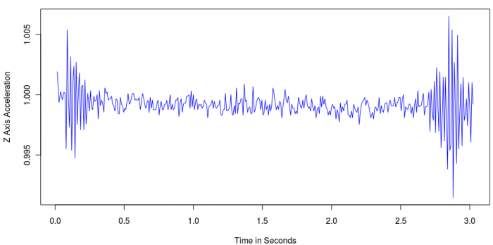
plot(data$Time,data$Accel_Z,type="l",xlab="Time in Seconds",ylab="Z Axis Acceleration",col="blue")

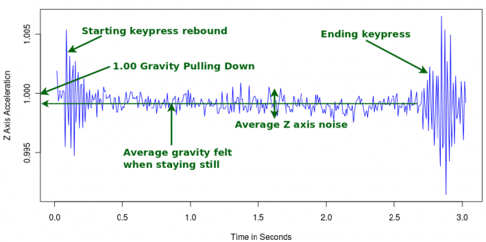
...Which produces a graph like this of our three seconds of recording:

Even from this little three second experiment, we have a number of events and data boundaries: